Map-Based Localization

Chapter 11 showed how SLAM turns raw scans into a registered point cloud. This chapter is about what that map is for. The map already exists. The question is how a robot uses it to determine where it is, and why getting the answer right depends on choices you make as a map builder.

When you build an HD map, you are not just tracing vectors. You are building the ground truth that every vehicle on the site will use, ten times per second, to answer the single most important question in autonomy: where am I right now?

Localization vs SLAM

SLAM solves two problems at once: mapping an unknown environment and tracking position within it. They are coupled: you cannot position against a map that does not exist, and you cannot build a map without knowing where you are.

Localization solves only the second problem. The map is given. The robot’s job is to find itself within it. This is an easier problem, with a harder requirement: the map must be right. If the map says a stop sign is at (45.2, 12.7) and it is really at (45.0, 12.8), every localization estimate that uses that stop sign will be shifted by the same 0.2 m. The robot will not know it is shifted. It will navigate confidently, 20 cm from where it thinks it is.

This is why Chapters 7 through 10 spent so much time on accuracy. A localization system is only as good as the map it localizes against. For a map anchored to the earth, the chain is survey accuracy → GCP accuracy → point cloud accuracy → map accuracy → localization accuracy. An error at any link propagates to the robot.

The Harbor Yard point cloud

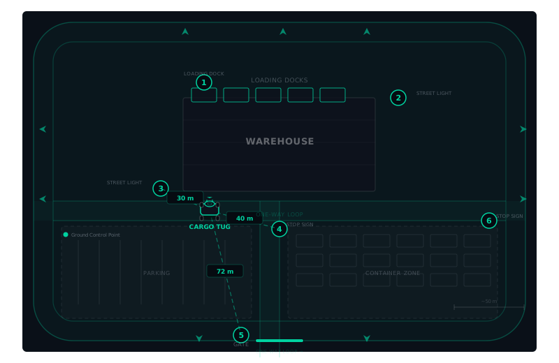
The site plan above shows the Harbor Yard point cloud in map form. A one-way loop encloses the yard, with a cross road and a vertical bisector splitting the lower half into parking and container zones. The circled numbers are fixed landmarks, features stable enough to be recognized across multiple scans.

The street light at (3), mounted near the southwest corner of the warehouse, is 13 m from that corner. The stop sign at (4), on the curb at the top-left corner of the container zone, is 58 m east. The gate at (5), a steel sliding barrier at the site entrance, is 87 m southeast. Barring a major earthquake, the street light will still be 13 m from the warehouse corner next week, month, and year. A measurement that does not go stale is a measurement a machine can rely on.

Why do fixed landmarks matter so much? They give the cloud texture. When a robot localizes in a future run, it matches its live scan against the saved point cloud, and it can only tell one place from another if the geometry there is distinctive. Landmarks, a pole, a sign, a dock corner, are the distinctive geometry. A cloud without them is accurate and useless at the same time: the robot has nothing to grab onto.

Suppose an autonomous cargo tug enters Harbor Yard. It carries a LiDAR scanner and a copy of the point cloud. It needs to know its position to within a few centimeters before it can begin its route. But GNSS in a yard full of metal containers and warehouse walls is unreliable. It might be off by 5 m, or 20 m, or more.

The tug scans the scene from the cross road. Its perception system recognizes three fixed landmarks: the street light at (3), the stop sign at (4), and the gate at (5). From the LiDAR returns, it measures:

Landmark	Distance from tug
Street light (3)	30 m
Stop sign (4)	40 m
Gate (5)	72 m

Three distances, three known positions. The tug solves for the one location consistent with all three: it is on the cross road, about 15 m east and 11 m south of the warehouse corner, facing the container zone. The whole calculation takes under a second. The position is accurate to within 5 cm.

That is localization in its simplest form: distances to known landmarks, solved for the one position consistent with all of them. Production systems do the same thing continuously and with raw geometry, and the rest of this chapter is about how.

How scan matching works

The robot carries a LiDAR scanner and a copy of the mapped point cloud. Ten times per second, the LiDAR captures a new scan, a sparse fan of points in the sensor’s frame. The robot needs to compute the rigid transform (X, Y, Z, roll, pitch, yaw) that places that live scan into the map’s coordinate frame.

The principle is simple. The robot guesses a pose. It projects the live scan into the map frame using that guess. It scores the match: how many live-scan points lie close to map points? It adjusts the guess and tries again. After a few iterations, the guess converges to the pose that best aligns the live scan with the map.

This is iterative closest point (ICP) again, the same algorithm used for scan registration in Chapter 10. The difference is speed. Registration runs offline, on a workstation, with the full point cloud. Scan matching runs online, on the robot’s computer, against a live stream of points arriving 10 Hz. The robot gets a fraction of a second per iteration.

To make this fast enough, most localization systems match features rather than raw points. A feature is a distinctive piece of geometry: a corner, a pole, a planar surface, a curb edge. Features are sparser than raw points but more informative. Matching a single pole base against the map constrains two dimensions (X and Y) simultaneously. Matching a planar wall constrains orientation as well as position.

The cargo tug at Harbor Yard does not match every LiDAR return against every point in the map. It extracts features from the live scan, narrows the search to the region around its last known position, and matches only against the mapped features in that region. The whole loop runs in under 100 milliseconds.

Autoware uses a different algorithm: the normal distributions transform, or NDT. Instead of matching individual points to their nearest neighbors, NDT models the point cloud as a grid of 3D probability distributions and scores how well the live scan fits those distributions. The practical difference for the map builder is small: both ICP and NDT need the same input, a clean, registered point cloud with enough distinctive geometry to constrain a pose. If you are building a map for Autoware, the localization step uses NDT by default. You do not need to implement it. You just need the point cloud to be good enough that the algorithm can find a match.

The accuracy envelope

Localization accuracy is not a fixed number. It depends on three things.

Landmark geometry. The triangulation above showed this: three landmarks at known positions produce a unique position solution to within a few centimeters. With two landmarks, the solution is ambiguous: the robot could be in either of two positions, mirrored across the line between them. With one landmark, the robot knows its distance from that landmark but nothing about direction. With zero landmarks, the robot is dead reckoning, estimating position from wheel rotation and IMU data alone, and the error grows without bound.

The number of landmarks matters less than their arrangement. Three landmarks in a line constrain position poorly perpendicular to that line. Three landmarks spread around the robot, as at Harbor Yard where the street light, stop sign, and gate form a rough triangle around the tug, constrain position well in all directions.

Sensor quality. A survey-grade scanner produces denser, more accurate returns than a mobile mapping scanner. More points per feature mean a better feature position estimate, which means a better pose estimate. The relationship is roughly linear: cutting sensor noise in half cuts localization error in half.

Map quality. This is the part the map builder controls. If the mapped position of a landmark is off by 10 cm, every localization that uses it is off by up to 10 cm. If the map is internally warped, a region where the SLAM trajectory drifted and was not corrected, the localization error varies across the site. The robot’s position jumps when it crosses from a well-registered region into a warped one.

Global vs local localization

Local localization assumes the robot knows roughly where it is, within a meter or so. This is the normal operating condition: the robot was localized a moment ago, it has moved a short distance, and it needs to update its pose. The search space is small and the solution is fast.

Global localization, also called the kidnapped robot problem, assumes the robot has no idea where it is. It could be anywhere on the map. The search space is the entire site, and the robot must match its live scan against every region of the map until it finds a match.

Global localization is much harder and much slower. A brute-force search of a 40-acre site at 10 cm resolution means evaluating millions of candidate poses. The feature-based matching described above narrows the search, but even so, global localization can take several seconds. It can fail entirely if the site has symmetries, regions that look identical from the scanner’s perspective.

Most operational systems avoid global localization by never losing track in the first place. The robot initializes its position at a known start point, typically a designated charging station or dock, and updates continuously from there. If localization is lost, the robot stops and waits for an operator to provide an initial pose estimate. This is not a software failure. It is an operational design choice: global localization is fragile, and a moving robot that does not know where it is is dangerous.

When localization fails

Localization fails in environments where the live scan does not provide enough distinctive geometry to constrain a pose.

Featureless corridors. A long, straight hallway with uniform walls. The scanner sees two parallel planes. That constrains lateral position and orientation, but not longitudinal position: every meter of the corridor looks identical to the scanner. The robot knows it is in the corridor and aligned with it. It does not know how far along it is.

Open pavement. A large, empty road surface with no curbs, poles, or markings in range. The scanner sees a flat plane below it. That constrains height and roll/pitch, but nothing about X, Y, or yaw. The robot could slide in any direction without changing the scan.

Symmetrical structures. At Harbor Yard, the container zone in the lower right is a grid of identical shipping containers. A scanner in the middle sees container walls in four directions. That constellation matches several positions equally well. The robot picks one, and if it picks wrong, it is offset by exactly the container spacing. The same trap appears in any parking lot with identical light poles in a regular grid.

The common thread is ambiguity: the live scan is consistent with more than one pose, and the robot cannot distinguish them. The map builder’s job is to reduce ambiguity by ensuring the map contains enough distinctive features, and enough of them, that every place the robot will go produces a unique sensor signature.

This is decided at capture time, not at runtime. When you plan the survey (Chapter 8), make sure every place a robot will drive has enough fixed landmarks in view to be recognizable. A bland region is not a region the robot reads less precisely. It is a region the robot gets lost in.

The map quality feedback loop

A bad map produces bad localization. If the bad position estimates feed new sensor data back into the map, the map gets worse. The worse map produces worse localization. The loop diverges.

This is why the fixed landmarks in Chapter 11 are fixed. They are the constants that prevent the loop from running away. A stop sign embedded in a concrete curb at a surveyed position is ground truth. The robot can use it to correct its position, and it can use its corrected position to observe that the shipping container in front of the warehouse has moved since last week. The fixed landmark anchors the system. Everything else can move relative to it.

The map builder who understands this loop makes different choices: more fixed landmarks, surveyed more carefully, positioned where robots will see them often. Each one is a reset button for accumulated error.

What comes next

Part III is complete. You now know what a point cloud is, how to capture and clean one, how SLAM produces a registered cloud from sensor data, and how a robot localizes against the finished map.

Part IV begins the next stage of the pipeline: Representation. How do we turn geometry into meaning?